Carlin Eng

Former Data Engineer and Engineering Manager at Strava; then spent two years as a Sales Engineer and Data Scientist at Snowflake. Currently working on the Malloy language at Google. Avid cyclist, and proud member of the Dolphin Club in San Francisco, California.

Made with 🚴‍♂️ by Carlin Eng

About

This page is based off of the John Doe template, a single-file website written only in HTML and CSS, to which I've added small Javascript snippets for toy functionality. Source code for this website can be found at Github. ↩️

[link]

There is no shortage of opinions on the Internet about how best to organize data: star schemas, OBTs (“One Big Table”), slowly changing dimensions, and Activity Schema, just to name a few. However, despite the existence of all these “best practices”, most data practitioners I know still describe their data warehouse as a complete mess. The most innocent question of “why are these two numbers different?” can send an analyst or data engineer down a deep rabbit hole for hours or days. With so much discourse about data modeling, why are we still in such a fragile situation? In this post, I argue that the root cause is the unnatural division of “data modeling” into two separate workflows: transformation and semantic modeling.

It's worth taking a second to discuss what data modeling actually is. Here’s my best attempt at a definition: “The process of turning raw data into useful business insights.” While this definition is broad and perhaps a bit too generalized, I’ve noticed that much of the online discourse seems to focus on specific tools or techniques. Some people talk about data modeling in terms of the artifacts it produces, for example, the aforementioned star schemas and OBTs. Others talk about data modeling as a way to map already-existing database objects to business metrics – what tables and columns feed into the revenue calculation? What segments can we cut revenue by? These two viewpoints correspond to two related, but mostly separate camps: data transformation and semantic modeling. Data transformation uses tools like dbt to define pipelines of SQL queries. These queries take raw data from business systems as input, and produce “clean” tables and views for downstream consumers to use. In the other camp, semantic modeling uses tools like LookML to specify joins between tables and define how measures are calculated from those tables.

A very common workflow is to use dbt to create pipelines that produce clean output tables, then use those clean output tables to generate metrics for reporting. These metrics can be defined either in a semantic modeling layer like LookML or directly in a visualization tool like Tableau. In either case, it’s rare for the transformation layer to own 100% of the metric logic. There are usually too many dimensional cuts and edge cases to enumerate explicitly in the pipeline.

At first glance this might seem like a reasonable approach, but let’s look at what happens when the inevitable question arises: “why is Number X different from Number Y?” Numbers X and Y probably come from two different dashboards, and if you’re lucky enough to use a tool like Looker, you can easily inspect the semantic layer to find the measure definitions that generated them. This is great, until you hit a wall: measures X and Y are built on tables that are “clean output tables” from a dbt job. Looker has no idea where those tables came from or how they were calculated; it just sees the materialized tables in the database. To understand the logic behind the columns where measures X and Y come from, you need to jump into dbt and trace the pipeline that generated their input tables. There is no longer a single place to look up how a metric is defined – the business logic for numbers X and Y is split across two tools that use different languages (SQL and LookML), and might not even be owned by the same team (BI team owns the BI tool, data engineering team owns the transformation tool). If this is the case, good luck in your quest. Crossing team boundaries can mean adding hours or even days to a task.

Transformation and semantic modeling are not fundamentally different tasks – they are two parts of the same process: turning raw data into business insight. And yet, our ecosystem forces them to happen in separate places, oftentimes with tools operated by separate users.

This problem has been recognized by many in the industry, but existing solutions all fall short. Looker’s Persistent Derived Table functionality allows users to construct data pipelines to materialize their models, but practically speaking, the resulting tables are really only usable by Looker, and are difficult to query directly from the data warehouse. dbtLabs’ acquisition of Transform is a sign that they have an intuitive understanding of the issue, but I’m not confident that their current direction will improve the situation. While full details of the integration haven’t been published, early indications are that it will look very similar to the workflow described above with all its flaws: SQL+dbt for transformations, and a YAML-based configuration language for semantic modeling. Still two separate languages and two separate toolsets for what is essentially the same problem.

Is there any solution to all of this? I can’t say for sure, but in my dream world, transformations don’t create tables or views, they create Models. Models are simply tables with additional metadata attached: joins, dimensions, measures, and more. Even further, every intermediate node in a pipeline DAG should also be a Model with the same types of metadata attached. Every Model should be queryable by BI tools, operational applications, or human analysts using a query language that understands the Model metadata. In such a world, the artificial divide between transformation and semantic modeling no longer exists, two tools get integrated into one, and the question of “why are these numbers different” becomes a lot easier to answer.


Discuss this post on Hacker News

[link]

Disclaimer: this blog post relates directly to my work as a Product Manager at Google; however, all opinions expressed here are my own and do not reflect those of Google. I also can't comment on any future Google product plans.

Semantic layers, also known as metrics layers or “headless BI”, have become a popular topic in recent years. The idea of a semantic layer is straightforward but powerful – put simply, it’s a system that takes tables in a SQL database and provides business context around them. A semantic layer can help answer surprisingly complex questions like “what is the exact definition of revenue?” Such an innocent question might require a lot of background knowledge to answer: what tables contribute to revenue, and how are they joined together? Which columns are the right ones to use, and which rows must be filtered out? It’s the job of a semantic layer to store all of this knowledge, so anyone can ask the question “what is revenue”, and not need to know all the arcane knowledge about the underlying dataset in order to answer it.

This is an old idea, present in many enterprise ecosystems (e.g., Microsoft, SAP), but in modern cloud data warehousing environments, semantic layers are always tightly coupled to a visualization layer. The BI tool Looker, with its LookML configuration language is a prime example. Much of the recent buzz around this topic relates to decoupling the semantic layer from the visualization layer, which would allow many other types of applications to leverage centrally defined metrics. Example use cases include customer segmentation for marketing campaigns and lead-scoring in a CRM. Benn Stancil called the semantic layer “the missing piece of the modern data stack”. In a post titled Headless Business Intelligence, Ankur Goyal and Alana Anderson predicted that it would be the foundation of “the next generation of software companies“. Airbnb made a big splash with a blog post describing its internal metrics layer, Minerva. All these articles generated a fair amount of excitement in the online data community, but despite all that, we have yet to see this supposedly transformative idea change our profession. Several startups gave it a shot (Transform, Supergrain, Cube, and more), but haven’t seen much traction amongst analysts. Transform was recently acquired by dbt Labs for an undisclosed amount, Supergrain has pivoted, and Cube explicitly targets developers rather than analysts. So why has a concept that seemed to resonate so deeply with so many in the data community failed to take off?

Querying a Semantic Layer

To begin, I’ll defer again to Benn Stancil, co-founder and CTO of Mode Analytics, when he asks “Is Minerva the answer?”

My biggest gripe with Minerva is how you “query” it. As best I can tell, metrics are extracted from Minerva via API; [...] it looks like the API lets people request metrics over date ranges, with filters, and grouped by different dimensions.

[...] API-based solutions don’t work for analysts working directly in SQL. Though I don’t know how analysts work at Airbnb, in the broader market, most analysts’ work starts in SQL; for many, it also ends there. Unfortunately, Minerva appears to be inaccessible to these workflows. Analysts, when inevitably asked to explain why some KPI is yo-yoing across a Minerva-backed dashboard, will eventually have to recreate that metric, in SQL, on raw data in their warehouse.

Benn hits it right on the nose. Querying these models takes an analyst out of their most familiar tool (SQL) and forces them to use an API, shunting them into tools like Python or R to carry their analysis further. If they hit a snag (e.g., numbers don't match, or things look wonky), they're forced back into the world of raw SQL without any of the benefits of the metrics layer, and stuck with the unpleasant task of resolving differences between hand-written and machine-generated SQL. But even assuming the happy path, once in Python-land the analyst is hamstrung in the following ways:

  • Analytical freedom is severely limited. Since data from the metrics API is already aggregated, there’s no way to drill into specific records, or create on-the-fly dimensions and measures to slice the data in a way that might reveal new insight. You can request other dimensions from the metrics layer, but what if the dimension you’re interested in doesn’t exist yet?
  • The analyst is now constrained to whatever environment is hosting their Python runtime, whether that’s a local laptop or a cloud-hosted notebook. Operations that require more memory or compute aren’t possible.
Clients of these metrics layers are isolated from the data warehouse, and only able to communicate with the warehouse via a very restrictive API. This might be sufficient for a subset of an analyst’s work such as building executive reports and dashboards, but it falls flat when the analyst needs to do critical work like debugging misbehaving metrics, or more creative data work such as exploratory deep-dives.

Model Development

We’ve looked at the metrics layer from the perspective of an analyst, but what about a data modeler? Suppose you want to define a new metric or dimension… what does the workflow look like? I imagine something like the following:

  1. Write ad-hoc SQL queries against the data warehouse to develop the metric
  2. Once the SQL logic has been validated, edit a YAML configuration file to encode this logic in the semantic layer
  3. Push the new configuration to source control, potentially get it code reviewed
  4. Redeploy the semantic layer service, or trigger data pipelines to calculate the new metric
  5. Get a coffee
  6. Fire an API call to the semantic layer to get your metric, and confirm that it’s actually what you want
Steps 2-5 have the potential to take hours, and step 6 takes the analyst away from their most familiar language. If there’s a bug in the metric logic, or something else in the process goes wrong, iterating is painfully slow and requires context switching between SQL, YAML, and API. In summary, in order to solve the problem of consistent business logic, semantic layers like Minerva take an analyst’s primary tool (SQL) and break it out into three parts that don’t play well together: SQL for exploration, a modeling language for definitions (typically YAML), and an API to interact with the data model.

Enter Malloy

I recently joined a team at Google trying to solve these issues. We’re building a new open-source language that offers a better way, and it’s called Malloy. Malloy unifies the semantic layer and the query language. Instead of writing exploratory SQL, developing YAML config, then making API calls, you simply write and execute Malloy. Malloy compiles to SQL, which runs directly on the data warehouse. This gives you the superpowers of a semantic layer, without sacrificing the freedom to explore, manipulate, and drill into the full unaggregated dataset.

To see an example that illustrates the point, check out this interactive Malloy notebook. It runs directly in your browser in Github's browser-based VSCode environment, github.dev. Once your VSCode environment has loaded in your browser, install the Malloy extension, and navigate back to the notebook file. The notebook demonstrates an example of building up a data model, using that model to explore and drill down into the raw data, and using insights from that exploration to iterate further on the data model. This sort of workflow is only possible when the semantic layer and the query language are the same, unified experience.

At first glance, it may seem like an impossible task to convince people to learn a new query language. After all, SQL has been around for over 40 years, and it’s “good enough”, right? Wrong. The excitement around metric layers struck a nerve because SQL is clearly NOT good enough. However, most iterations of metrics layers up until this point have provided a solution with too grave a cost. They completely fragment the analyst workflow and ask users to learn not one, but TWO additional languages: the metric configuration language and the metric API (an API is not so different from a small language, after all). With all that in mind, it’s not surprising that the metrics layer hasn’t taken off.

This is why I’m so excited about Malloy. It fulfills the promise of the metrics layer at a fraction of the cost. Plus, if we’re going to ask users to learn a new language, we can seize the opportunity to design it thoughtfully, incorporating everything we’ve learned from the past 40 years of working with data. After all, language is a tool for thought, and improving the syntax of a language has deep implications for what we can imagine and what we can express.

If you’d like to learn more about Malloy, check out the Quickstart repository and our documentation. We also have a community Slack channel, where you are welcome to post any questions or feedback!

[link]

I’ve been writing a lot recently about Malloy, an experimental analytical query language built by members of Looker’s founding team. Upon reading the overview materials and documentation, it sounded like exactly what I was hoping for, but in order to develop a more informed opinion, I needed to get some experience with actually writing the language. Hence, I decided to embark on a project to translate each of the 99 TPC-DS benchmark SQL queries to Malloy. This post will give an overview of the TPC-DS dataset, the queries, and the opinions I've formed about Malloy along the way. For a more introductory overview of Malloy, check out my prior blog post, as well as the Malloy documentation.

I posted the translations of all 99 queries to this Github repository. If you'd like to try any of these out for yourself, it's trivial from within the github.dev web editor. Simply go to "Extensions" in the lefthand sidebar of the editor and install the Malloy extension. The Malloy queries will then be runnable directly in your browser by clicking on the "Run" button above any query. Give it a shot with this query!

A Brief Overview of the TPC-DS Benchmark

TPC-DS is a well-known standard for benchmarking the performance of OLAP database systems. From a paper entitled “The Making of TPC-DS”:

“TPC-DS models the decision support functions of a retail product supplier. The supporting schema contains vital business information such as customer, order, and product data. The imaginary retail company sells goods through the three distribution channels, store, catalog and Internet (web).”
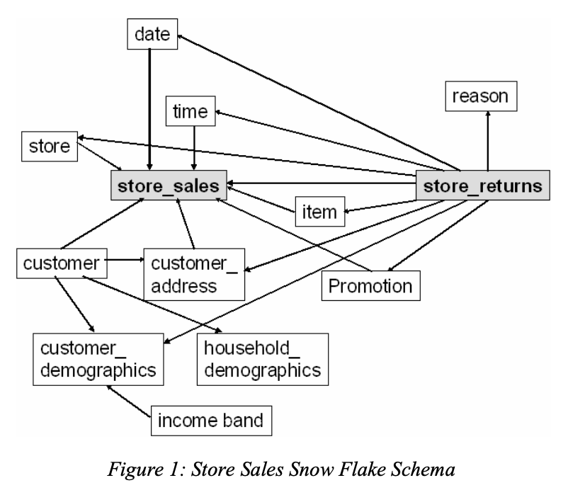
The benchmark contains 99 SQL queries of varying complexity against a star-schema data model containing 7 fact tables and 17 dimension tables. This sample schema diagram describing a portion of the data model has been taken from the paper above:

The queries test a wide range of OLAP query functionality as specified by the SQL99 standard, including common table expressions, ranking window functions, and joins of all types. Because of this, it is considered by many to be a “completeness” test for a query engine’s capabilities. For example, as of February 2023, Altinity’s benchmark repository reports that Clickhouse currently only passes 75% of the queries. Based on this reputation, I thought the query suite would make a great case study in testing the capabilities of Malloy, as well as giving me the opportunity to develop a firsthand perspective on the language.

Getting Acquainted with the TPC-DS Queries

Though I had previously read a lot of TPC-DS benchmark reports and looked superficially at some of the queries, I didn’t actually know the queries or the schema all that well. It didn’t take long for me to realize that the benchmark is far from a picture-perfect dataset with cleanly written SQL. Some of the queries contain bugs, the data model is not always applied consistently, and the SQL style employed by the authors is somewhat unconventional.

Bugs in Queries

Several of the queries contain exploding joins due to poorly specified join conditions between tables. In some queries, like Query 2, the results contain duplicate rows that provide no meaningful information. In another example, Query 54, one of the joins (store and customer_address) causes a fan-out followed by a sum on duplicate rows, ultimately generating an incorrect result. In Query 77, one of the joins is simply missing any join conditions at all, which results in an aggregation on top of a cartesian join, again producing incorrect results.

Inconsistencies in Data Model Between Queries

In Query 49, the join condition between the store_sales and store_returns tables uses two columns, item_sk and ticket_number. In Query 17, the join between the tables includes a third column, customer_sk. It’s possible that there’s a legitimate reason why one query should use a different set of join keys than another, but this is exactly the sort of arcane knowledge that is likely to cause bugs when working in a complex data warehouse. When encountering these tables for the first time, how does an analyst know which join keys are appropriate for which situation?

Other Miscellaneous Issues

Join Specification: The majority of joins are specified in the WHERE clause instead of using the JOIN keyword. I dislike this syntax because I think it makes queries harder to interpret. I prefer to structure my SQL queries such that each part of the query is associated with a particular “action”, e.g., joining, grouping, aggregating, or filtering. Using the WHERE clause to specify joins means that filtering and joining operations can be interleaved in the query text, and that the join condition is oftentimes far away from the names of the joining tables (see Query 25). This makes understanding the query just a bit more difficult since filters and joins can be hard to distinguish from each other. Understanding how the join occurs now requires jumping back and forth between different parts of the query.

Correlated Subqueries: A large number of the queries use correlated subqueries (e.g., Query 1 and Query 41). I’ve always found correlated subqueries hard to understand, since the join syntax requires joining a column in the subquery to an “outside” column, which oftentimes lacks immediate context to indicate where it comes from. This forces the reader to backtrack (oftentimes quite far) to earlier in the query to figure out what’s going on.

GROUP BY ROLLUP: A lot of the queries use the GROUP BY ROLLUP construct (e.g., Query 18). While most modern data warehouses support this functionality, I’ve very rarely seen it used in practice because the output is so clumsy and difficult to work with. For more on this topic, check out my prior blog post.

To be fair, most of the above issues are quite likely to appear in a real-world data warehouse. It’s not unreasonable for a benchmark suite to contain problems like these, but I doubt they were intentional. I couldn’t find any mention of intentionally including mistakes when I browsed through the TPC-DS reference materials.

Translating to Malloy

The Malloy language currently supports querying Postgres, DuckDB, and BigQuery. I opted to use DuckDB because of the ease of setup — it’s an in-process database that doesn’t require running a separate server or a connection to the Internet, and it operates directly on local files.

Once I had the database up and running, writing the actual queries was pretty straightforward. The examples in the Malloy documentation provide a great template for getting started. I created a “model file” to develop the data model with predefined joins, commonly used aggregations, and other reusable constructs. Each individual query file imports this model file and uses one of the Sources defined there as a starting point for querying. Of the 99 queries, I was able to write logical translations of all but one: Query 51, which requires cumulative window functions. Of the 98 translated queries, 96 returned successfully with correct answers. One query failed due to a bug where the Malloy-to-SQL compilation process generated invalid SQL (Query 14), and the other was due to DuckDB crashing on the compiled SQL (Query 64). Given that the TPC-DS queries are considered a “completeness” benchmark for logical capabilities, I was rather impressed with Malloy’s coverage. 97% (96 out of 99) is solid, especially for a project so young.

In total, the Malloy queries consisted of 4,727 lines, 13,788 words, 129,880 characters. The SQL queries from the DuckDB repository are 5,524 lines, 14,961 words, and 184,424 characters. In lines of code, the Malloy is about 15% more compact, and over 30% more compact when looking at character count. In addition to being more concise, I’ve found the Malloy queries to be quite a bit more readable. Query 4 is an extreme example -- the SQL query comes in at a whopping 119 lines of code. Parsing a single 119 line SQL query is a task that requires a good deal of mental focus. The Malloy equivalent is only 37 lines:

It’s not a completely fair comparison, since the Malloy query leverages pre-defined logic imported from the model file, but even with that in mind, I find the difference between the two implementations quite informative.

Overall, writing Malloy queries is a lovely experience. Coming from SQL, the syntactic structure of the language feels familiar, but much more refined — as if the clunky, jagged edges of the language have been reshaped and sanded down, leaving something with a much smaller footprint, and a much more pleasing ergonomics. Malloy’s syntax seems smaller and has a more explicit structure. Unlike SQL, it doesn’t make the hopeless attempt to mimic human language, and seems instead optimized for someone trying to manipulate data using a well-understood set of actions — grouping, joining, aggregating, and filtering.

Interestingly, the explicit structure imposed by the language meant that I settled in very quickly on conventions for formatting my Malloy queries. When writing a query, there are far fewer formatting decision points than in the equivalent SQL query. While this may seem trivial at first, it’s a subject that has spawned a number of linting packages, and more than a few essays by analytics influencers. Reducing the time spent picking apart query formatting means more mental energy can be spent on the logic itself. This is a much improved experience for writing queries, and even better for reading them. There are countless examples of this in the TPC-DS queries, but Query 4 above is a prime example. The SQL query contains filters with nested case statements, UNION ALL statements, and common table expressions. With each of these elements, formatting is applied inconsistently, and it took me a good deal of time to piece together the logic. The Malloy version is clearly much more concise and far less chaotic.

Drilling into a few more details, here are some additional points where I found Malloy to be a clear improvement over SQL:

Joins: the ability to leverage a pre-defined data model and not have to remember and write out join keys for every single join was really great.

Nested Aggregations: Nested aggregations take the place of GROUP BY ROLLUP, and do a far better job (see Query 22). As mentioned previously, see my previous blog post for a deeper dive on this topic.

Filtered Aggregations: Filtered aggregates are so much nicer to use and interpret than using CASE statements inside aggregate functions (see Query 21). Some SQL databases have implemented this functionality, and I think it’s a no-brainer to make it a standard part of the language.

Potential Areas for Improvement

While the experience was overwhelmingly positive, there were still a few spots where I fell into traps, or where the language didn’t feel quite optimized for the task.

LEFT JOIN vs INNER JOIN: All joins in Malloy are LEFT JOINs by default. To implement INNER JOIN semantics, a query needs to specify a filter on right_table.column = null, which I would often forget to do. It’s trivial to add these filters, but in SQL queries, the type of join is a critical piece of information that is oftentimes the first thing an analyst will look at to determine the nature of a query. Having the INNER JOIN indicator placed in a `where` clause might not be obvious to someone quickly glancing at a query, since `where` clauses are typically reserved for filtering down datasets based on properties. From a UX perspective, since joins in Malloy are usually defined in a Source and not necessarily the query itself, it’s not clear to me how to make this more obvious, and it might just be one of those things that takes some getting used to with a new tool.

SEMI-JOIN: The semi-join operation in SQL takes the form of WHERE customer_id IN (SELECT … FROM …), as seen in Query 33. The Malloy implementation of this construct requires an extension to a Source with an ad-hoc join (lines 2-7 in the query below), and an additional NULL filter in the where block (line 16):

Logically, this produces the correct output, but I don’t love the syntax since it combines two operations that could each have separate semantic meanings, and which are far apart in the query. This makes it harder to interpret exactly what the query is doing. By contrast, the SQL syntax of column IN (sub-select) is neatly contained in a single location, and unambiguous in its intent.

Conclusion

Throughout this entire process, I learned a lot about both Malloy and the TPC-DS benchmark. Initially, writing 99 queries in a new query language felt like a huge task, but it wasn’t long before I hit my stride. The Malloy language made the task easy, and dare I say, fun. Getting up close with the benchmark queries was hugely educational as well. The dataset and queries are impressive in many aspects, but ultimately, I don’t think they’re very representative of actual workloads. Even though it has earned a reputation as a coverage test for a query engine’s logical completeness, there are still many real-world query patterns and scenarios that are not represented, such as session analysis, or the construction of “date-spined” reporting tables. As a result, I’ve come away from the exercise more excited about Malloy than ever, but acutely aware that there is still much to be tested. Will Malloy ever truly replace SQL as the lingua franca of the analytics world? If it does, it will take a long time to get there, but it’s a future I’d like to live in.

[link]

This post is the third in a series comparing SQL with a promising new query language called Malloy. I think Malloy represents a leap forward in how we work with data, and in the following paragraphs, I'll attempt to draw a connection to another time in history of rapid technological advancement: the Renaissance in Western Europe.

Lloyd Tabb, former Looker CTO and creator of Malloy, recently wrote a post entitled Data is Rectangular and Other Limiting Misconceptions. If you haven’t read it yet, go check it out now — it very neatly lays out a fundamental flaw in SQL’s perspective of data, and describes how the Malloy language does better. In particular, SQL resultsets can only naturally represent data in two dimensions: rows and columns. However, data in the real world is NOT two-dimensional. This mismatch results in awkwardness in both writing SQL queries and interpreting SQL results. As I was reading Lloyd's post, it sparked a memory of a recent trip I took to the Uffizi art gallery in Florence, Italy.

The Uffizi is the former administrative office of the powerful Medici family that ruled Florence during the 15th century. It currently houses one of the world’s largest collections of Gothic and Renaissance art, spanning from the 12th to the 16th century in Western Europe. I personally have minimal knowledge of art and art history, but the tour we took highlighted some fascinating aspects of technological advancement during this time.

Gothic Art

Gothic paintings such as this depiction of the of the Virgin Mary, attributed to Florentine painter Cimabue circa 1290-1300, were flat scenes with close-up figures in the foreground. The notion of perspective had not yet been developed, and rather than attempt to create images with depth, many paintings filled the background with gold leaf, which served as a representation of heaven.

Transitioning to the Renaissance

The transition from the Gothic to the Renaissance period was marked, among other things, by a growing understanding of perspective: the ability to accurately represent three-dimensional scenes on a flat canvas. The Battle of San Romano by Paolo Uccello circa 1435-1440 is a great example from this transition period. A fierce battle rages in the foreground, while scenes from life in the Italian countryside play out in the background. Uccello clearly understood that far away objects in the background must be smaller than those in the foreground, but just how much smaller hadn’t been fully worked out yet. Look at the hunting scene in the background — the hunters and hares would be massively tall if brought to the foreground.

The Renaissance

Finally we arrive at The Annunciation by Leonardo da Vinci, painted around 1472-1476. Here, the lines of the building behind Mary clearly converge into a well-defined vanishing point in the background. The mountains, ships, and trees behind the kneeling archangel Gabriel appear realistically distant. This was as much a technological advancement as an artistic one. Da Vinci applied his knowledge of mathematics to accurately represent the three-dimensional world on a two-dimensional canvas.

SQL: The Gothic Art of Query Languages

A SQL resultset is a two-dimensional canvas with rows on one axis and columns on the other. The typical star-schema data model contains hundreds of dimensions which can be used to slice, dice, and aggregate data. Because a SQL resultset can only naturally represent two dimensions, any single projection of the star-schema model can only represent the data in two dimensions. A query that aggregates along a single level of granularity is like the Gothic painting above -- a flat scene representing two dimensions, without any notion of depth. Queries that require aggregation at different levels of granularity (like the hierarchical subtotals of my last post) are possible, but fit awkwardly into the two-dimensional output of the query. Looking at the results of a GROUP BY ROLLUP query is akin to looking at the Battle of San Romano. The point comes across, but the image is contorted and unnatural.

Malloy: A Query Language Renaissance?

Malloy’s approach breaks free of the two-dimensional constraints of rows and columns by allowing columns to take a “table” type. This means sub-tables can be nested within a single column, and hierarchies can be preserved. By allowing sub-tables within resultsets, Malloy results are able to faithfully represent the true dimensionality of the underlying data. The idea of nested tables is not a new one. Database researchers have discussed this idea of "relation-valued attributes" since at least 1986, but no relational database on the market supports them natively.

I described the following example in depth in my previous post, but to quickly go over it again, the following SQL query generates a result aggregated at both the yearly and monthly level.

Note that data aggregated at the yearly level is duplicated in every row. This column is now "unsafe" for use by downstream queries. Summing the yearly_sales column will result in values that are wildly incorrect.

Compare this to the equivalent Malloy query:

The by_month column contains a nested table, with its own rows and columns, and we no longer have duplicated data for yearly sales.

This is more than just an aesthetic improvement. From a practical standpoint, any Malloy result can be plugged into downstream computations without worrying about the necessity of arbitrary filters or falling into the fan/chasm traps. The importance of this cannot be overstated! Writing a query the "obvious" way in SQL will oftentimes result in something that is syntactically valid, but semantically meaningless. I believe this is a major deficiency of the tools we use. The "obvious" way should be the correct way, and anything less is a serious design flaw.

[link]

In a previous blog post, I wrote about Malloy, a new language for querying analytical databases. My main argument was that the killer feature of Malloy is its integration of a semantic layer inside an interactive query language. The discussion on Hacker News was, as expected, quite lively, and provided great food for thought. This post is a response to some of those comments, an exploration of some of the deficiencies of SQL's syntax, and a demonstration of how Malloy gets it right.

A lot of those comments were along the lines of:

SQL + recursive queries is Turing complete. Thus every arrangement and selection of data is reachable by a query. Therefore there is nothing Malloy can do that SQL can't (I'm absolutely sure of it).

and:

I don't see much value in this. This is not aesthetically better than SQL. It's also not semantically better. This is just a different syntax that would parse to the same AST.

Both of these comments dismiss Malloy, pointing out that one can write semantically equivalent queries in SQL. While they are technically correct that Malloy queries all have semantically equivalent SQL queries, this misses a critical point: the syntax of a language has a profound impact on what users of that language choose to express. As the saying goes, “first we shape our tools, then our tools shape us”.

After over a decade of using SQL nearly every day for data analysis, I’ve developed a strong conviction that SQL’s syntax is not just awkward and annoying, but actively harmful. By making certain types of queries difficult to write and interpret, it trains users to avoid asking those questions. In this thread, some commenters take on the challenge of implementing a SQL equivalent to a Malloy query. However, I think the relevant question is not “can you write a SQL query that answers question X?”, but rather “would you have thought to ask question X in the first place?”

This speaks more broadly to a common dissatisfaction I see amongst analysts and data scientists. Many analytics jobs are essentially writing SQL queries to answer questions from higher-ups. Data lies at the bottom of a mystical lake, and only the analyst knows how to mutter the right SQL incantations to retrieve it. However, when the time comes for the analyst to ask their own questions, the first ideas that will likely come to mind are ideas that are easy to express, and not necessarily those that are most impactful or creative. I suspect this is especially true in cases where the analyst does not have deep domain expertise, and operates in a centralized “ticket-taking” support model. The syntax of SQL subtly guides a user’s mindset towards answering particular types of questions, and avoid answering others.

A Simple Example: Nested Analysis

A concrete example of something difficult in SQL is any kind of nested analysis, such as computing subtotals and percent of total in a hierarchical dimension. For example, suppose we have a table of daily sales, and we want to roll up total sales simultaneously at the monthly and yearly level:

This is typically done in SQL with one of three approaches: (1) computing multiple subqueries and joining the results together, (2) using a window function to aggregate at different levels, or (3) using a GROUP BY ROLLUP clause, if supported by the database. The queries for each of these approaches is below:

Each of these three options produces a correct answer, but presented in a seriously flawed way. A query like this requires the data to be aggregated along multiple grains (year and month, in this case); however, a typical SQL query is only capable of naturally representing data in two dimensions (rows and columns), which corresponds to one level of granularity. To represent more than one level of granularity, a query must resort to unnatural representations that are difficult to interpret and use. This is tough to explain in words, but hopefully the following examples are more clear. In approaches (1) and (2) above, the SQL results contain duplicate data for the coarser grain (yearly sales):

The yearly_sales column above contains duplicate data for each month's row. Doing a naive SUM(yearly_sales) aggregation on this table is a dangerous operation that will lead to incorrect results without the appropriate filters.

In approach (3), yearly aggregates are represented as rows where the finer-grained column (month) contains NULL values:

Values aggregated at different grains are all contained in the total_sales column. Whether it's a yearly aggregate or a monthly aggregate depends on the values of other columns. Here again, running SUM(total_sales) is potentially a very dangerous operation.

In all of these cases, the resulting “sales” columns can no longer be used as inputs to aggregate functions or other downstream transformations, since the rows contain duplicated information. If this table is consumed by downstream queries, those queries must take extreme care to apply the appropriate filters or transformations to prevent duplicates from entering the calculations.

The Malloy Way

The nesting functionality in Malloy allows you to write a subquery within an aggregation. This will produce a sub-table for each row in the GROUP BY clause. It feels much more natural to write the query this way, since the query is now written in a way that matches the hierarchical logic that’s being performed:

The output is presented in a way that respects the hierarchical relationship of the data. Every aggregate column contains data at a single level of granularity, and we no longer see duplicate values for data at the coarser grain.

This is possible because the by_month column in the result set of this query is of type struct, which effectively contains a sub-table. The Malloy VSCode extension renders this struct data as if it were just another table. This is easier to write, easier to interpret, and avoids all the pitfalls of the equivalent SQL implementation. The output of this query can be used naturally by any downstream queries or analyses without having to worry about hidden traps.

It’s a pretty simple example, but I think it illustrates the point nicely. In my career as a SQL monkey, I’ve *been asked* to do analysis like this many times in the past, and its always been possible. But when looking at a dataset on my own, its rare that these are the first questions that *I will ask on my own.* I’m convinced that these syntactic improvements offer more than just enhanced productivity for the user, but enhanced creativity as well. To see what’s possible with more sophisticated examples, I highly recommend checking out some of the examples on the Malloy documentation site, or playing with the Composer application , a web app built on top of Malloy.

[link]

Follow along with the discussion at Hacker News.

The foundations of SQL were laid at the dawn of the relational database. Back then, there was no such thing as a data warehouse, no such thing as a BI tool, and certainly no such thing as an Analytics Engineer. And yet, SQL is still the primary user interface by which most data professionals interact with their raw materials. The underlying technologies have improved immeasurably, but aside from a handful of updates to the ANSI standard, the core of the language remains untouched. It’s practically a miracle that after 40+ years of use by countless data professionals, our interface to data is effectively the same.

Since its inception, many computer scientists and database researchers have expressed their disdain for SQL, and their critiques are usually well-founded; however, every serious attempt to replace it as the de-facto standard has failed. Most attempts to replace SQL primarily address the language’s awkward syntax; for example putting the FROM clause first or removing the need for HAVING and QUALIFY clauses. Unfortunately, the reality is that SQL is “good enough” for most use cases, and according to Aiken’s Law, programmer training is the dominant cost for a programming language. It seems that syntactic sugar is simply not enough to overcome SQL’s entrenchment.

This brings me to Malloy, a new query language for data analysis currently being developed by Lloyd Tabb, founder and former CTO of Looker. Malloy addresses many of the aesthetic concerns that plague SQL, but far more interesting in my opinion is its integration of a query language and a semantic layer into a single language. But what is a semantic layer, and why is it important?

Semantic Layers

A semantic layer’s purpose is to codify domain-specific logic on top of database tables, and to prevent users from issuing queries that are syntactically valid, but semantically meaningless. For example, what happens if you write a join between two tables with incorrect keys? In most relational databases, primary and foreign keys are just strings or numbers. Some databases may enforce referential integrity, but most will not complain if you attempt to join, say, CUSTOMER_ID with ORDER_ID. As another example, it’s often the case that primary key columns are integers, and databases will happily let you use them as inputs to any aggregate function that takes a number input, like SUM or AVG, even though the result is nonsense. Lastly, every organization has special rules that must be applied to their datasets in order to correctly calculate key metrics. For example, what inputs and adjustments go into calculating the revenue that Investor Relations reports out to Wall Street? Someone with access only to the raw data, but not the requisite domain-specific knowledge will not be able to accurately reproduce these metrics. The semantic layer provides a place to set these rules and require queries to abide by them; e.g., which joins are valid, which columns can be grouped on, or what inputs go into a particular aggregate function.

A semantic layer usually takes the form of an application that sits on top of the database, along with configuration files that define the rules described above. Examples of products on the market today include SAP’s Business Objects Universe, Looker’s LookML and Cube. I was an early user of Looker, and that experience left a strong impression. LookML allowed me to define the logic necessary to package all of our data sources together as a cohesive single source of truth. Our data warehouse turned from a tangled mess of tables that only a skilled data scientist could operate, into a trusted repository that the typical PM or business partner could pull insights from.

Despite the huge value we got out of Looker and LookML, the analytics and data science group never loved it as much as I did. In comparison with Tableau, Looker’s interactive data exploration and analysis capabilities are relatively limited, and most data scientists saw exploration and analysis as their primary activity. They viewed writing LookML configuration as a chore, and the user experience did not help. To add a new dimension or measure, a data scientist would have to edit a YAML configuration file, check their changes into source control, and reload their configuration before they could view any results. A simple workflow that could take 2 seconds in Tableau might take over a minute in Looker. When trying to explore a dataset, the ability to iterate “at the speed of thought” is critical, and that extra latency was a source of frustration for many. As a result, data modeling and data exploration were viewed as two entirely separate disciplines. Data scientists greatly preferred tools that aided the latter, much to the detriment of everyone who was NOT a data scientist.

Malloy

So finally we return to Malloy. As I mentioned previously, Malloy is a query language that compiles to SQL, and looks very familiar to anyone who has used SQL. The team has also built a VSCode extension that allows users to connect to a database and start writing queries, currently with support for BigQuery, DuckDB and Postgres. The semantic layer within Malloy is accessed via writing Sources. From the docs:

A source can be thought of as a table and a collection of computations and relationships which are relevant to that table. These computations can consist of measures (aggregate functions), dimensions (scalar calculations) and query definitions; joins are relationships between sources.

Let’s take a look at an example Source from the Malloy Github repo, looking at a database of flights.:

source: flights is table('duckdb:data/flights.parquet') + {
  primary_key: id2

  // rename some fields as from their physical names
  rename: origin_code is origin
  rename: destination_code is destination

  // join all the data sources
  join_one: carriers with carrier
  join_one: origin is airports with origin_code
  join_one: destination is airports with destination_code
  join_one: aircraft with tail_num

  // declare some resusable aggregate calculations
  measure:
    count is count()
    total_distance is sum(distance)
  }
}

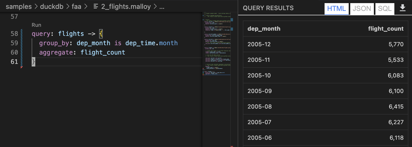
This Source has a few key components: the name of a table in the database, the primary key of the table, which tables can be joined to it and via which columns, and which aggregations (aka measures) are valid. Within the VSCode extension, I can use this source as the starting point for data exploration or analysis simply by writing a query referencing it, and hitting the “Run” CodeLens button:

The VSCode extension compiles the Malloy query to SQL, issues it against the database, and renders the results in another window.

That exploration may spur me to update the Source in some way, which I can do from right within the IDE, and immediately re-execute the query. This sort of read-eval-print loop enables fast iteration in a way that simply isn’t possible with LookML or any other semantic layer that requires both SQL and YAML for configuration (and even worse, oftentimes a separate API for actually querying the data). Malloy’s semantic layer marries two separate but intricately related disciplines – exploring data and codifying rules around it. This not only removes the overhead of context switching between the two tasks, but it actually improves the individual experience of each. Implementing a data model actively improves the data exploration experience, and vice versa.

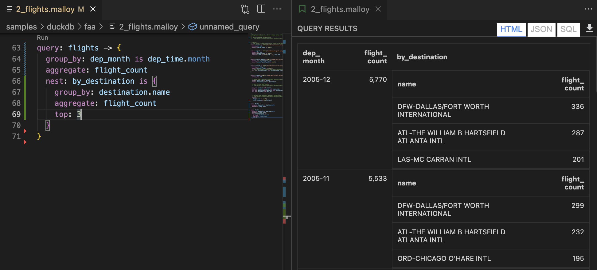
While the semantic layer is the main attraction for me, there are many other noteworthy features. One particularly nice feature is its handling of nested data. Rollup queries with nested subtotals can be painful to write in SQL, and the GROUP BY ROLLUP function in most SQL dialects produces awkward output that is very difficult to work with. Malloy’s nest clause makes this trivial. The previous query simply counts the number of flights by month. Let’s say I now want to compute the top 3 destination airports for each month:

For each row in the original by-month query, there’s a new column that contains a nested table with flight counts by destination. Note also that since the original flights Source has pre-defined the join with destination, accessing fields from the destination table is as simple as referencing them with dot notation: destination.name in the above example. Getting this same information in a single SQL query is quite a bit more verbose and requires either a window function or a self-join:

WITH flights_by_destination_and_month AS (
  SELECT
    DATE_TRUNC(‘month’, dep_time) AS dep_month,
    d.name AS destination_name,
    COUNT(*) AS flight_count
  FROM flights f
  LEFT JOIN destination d
  GROUP BY 1,2
)
SELECT
  dep_month,
  destination_name,
  SUM(flight_count) OVER (PARTITION BY dep_month) 
    AS flight_count_by_month,
  flight_count AS flight_count_by_dest_and_month,
FROM flights_by_destination_and_month
QUALIFY ROW_NUMBER() OVER (
  PARTITION BY dep_month ORDER BY flight_count DESC
) <= 3
ORDER BY 1,2

There’s a lot more to Malloy than what I’ve shared here, so I encourage you to take a look at the Github repository and the documentation.

Summary

Could Malloy finally be the language that replaces SQL? It’s a nigh impossible task, but I am very much hoping that it succeeds. Unlike other projects that only seek to improve on the aesthetics of the language, Malloy takes a more ambitious approach and tackles a critical missing piece of the stack. Its marriage of query language and semantic layer has the potential to radically change the disciplines of analytics and business intelligence for the better. Other trends, such as the rise and dominance of a few data platform products, namely BigQuery and Snowflake, mean that for Malloy to really succeed, there are relatively few database targets that it must support. It’s still very early days for the project, and who knows where it will go from here, but this is one that I’ll be keeping a very close eye on.

[link]

Author's note: this post has found it's way to the front-page of Hacker News -- follow along with the discussion there.

The SQL language made its first appearance in 1974, as part of IBM’s System R database. It is now nearly 50 years later, and SQL is the de facto language for operating the majority of industrial grade databases. Its usage has bifurcated into two domains – application programming and data analysis. The majority of my 12 year career (data engineer and data scientist) has been concerned with the latter, and SQL is by far the language that I have used the most. I love SQL for the productivity it has afforded me, but over time I’ve also become aware of its many flaws and idiosyncrasies. My perspective is primarily from a practitioner’s standpoint, and I have always been curious if those “real world” issues have more fundamental or theoretical underpinnings. This brought me to A Critique of the SQL Database Language, by mathematician and computer scientist CJ Date. Date was a former IBM employee, a well known database researcher, and friend of EF Codd. The SQL standard has received many major updates since this critique was first published, but which of those critiques are still valid today?

A Critique of the SQL Database Language was first published in November 1984 in The ACM SIGMOD Record. It examines the dialect of SQL implemented by several IBM systems (SQL/DS, DB2, and QMF) which provided the basis for the initial SQL standard. Having no direct experience with any of these systems, reading the SQL examples from the paper is a bit like trying to read 17th century English – it has a stilting, unfamiliar cadence that requires an extra bit of effort to understand. In the examples below, I’ll use the terms SQL[1983] and SQL[2022] to distinguish between the older dialect, and what is available today. Use of the unqualified term “SQL” means my comment could apply to both.

The paper consists of eight sections, each one describing a different category of criticism: lack of orthogonality in expressions, lack of orthogonality in functions, miscellaneous lack of orthogonality, formal definition, mismatch with host language, missing functions, mistakes, and missing aspects of the relational model. In the rest of this post, I’ll go through each of those sections, describe the critique in informal terms, and give my interpretation on whether the critique is still relevant.

Lack of Orthogonality: Expressions

Orthogonality with respect to programming languages means roughly that the constructs of the language are like Lego blocks – a small number of basic pieces can be recombined in simple and intuitive ways. Lack of orthogonality (again, informally speaking) means the language has lots of special cases and exceptions in how the components can be put together, which make it complex to learn and unintuitive to use.

This section begins with a definition of table-expression, column-expression, row-expression, and scalar-expression. Respectively, these are expressions in SQL that return a table, column, row, and scalar value. In SQL[1983], the FROM clause of a SELECT statement was restricted to only specifying table or view names, and not general table-expressions, i.e., subqueries or common-table expressions (CTE). This made constructing nested expressions, one of the key features of Relational Algebra, nearly impossible. Modern SQL provides the capability to reference a CTE or subquery in a FROM clause, so this concern is mostly irrelevant today; however, the idea that a table-expression can take the form of “tablename” in some contexts, but must be SELECT * FROM tablename in others is interesting.

For example, why not allow the following expression as a legal statement:

tablename;

which would return identical results to:

SELECT * FROM tablename;

Both are table-expressions (statements that return a table), and thus should be allowed anywhere that accepts a table-expression, e.g., the FROM clause of a SELECT statement, or a statement itself.

While SELECT statements in SQL[1983] are not allowed in the FROM clause, they are required as an argument to an EXISTS clause. Furthermore, the SELECT statement here is required to be a column-expression (selecting only a single column) – a statement that returns a table, a row, or a scalar will not work. When is a SELECT statement a table-expression, a column-expression, a row-expression or a scalar-expression? The language itself provides no guidance here, and it is wholly dependent on the query itself; e.g.:

SELECT a FROM tablename;

is a column-expression, but

SELECT a,b FROM tablename;

is a table-expression. This bit of arbitrariness still exists in SQL[2022].

Lack of Orthogonality: Functions

While some of the concerns in this section are mitigated by the introduction of subqueries and CTEs, a lot of them still hold true today. Column functions in SQL take a column of scalars as input, and return either a column of scalar values (e.g., the MD5 function or a type-casting function), or a single scalar (e.g., aggregate functions like SUM). The author argues here that since column functions take a column of scalar values as input, any valid column-expression should be allowed. An example where this is not the case is as follows:

SELECT SUM(val) FROM tbl

is allowed, but

SELECT SUM( SELECT val FROM tbl )

is not, even though SELECT val FROM tbl is a valid column-expression – it returns a single column, val, from table tbl.

The key problem here is that the input to the SUM function in the first example is a column name, but that column name alone does not define the column-expression. Instead, we must look at the context (i.e., the full query) to understand that the “val” column comes from “table”. Said another way, in SQL, F(X) is not dependent only on X, but on contextual information surrounding F:

SELECT SUM(amount) FROM purchases;

and

SELECT SUM(amount) FROM purchases WHERE 1 = 0;

Are two very different queries, even though the column-function invocation SUM(amount) is identical.

This also makes it difficult to nest aggregations. Consider the following example: we have a database of purchases for an ecommerce website, and want to retrieve (1) the total amount spent for each customer, and (2) the average spend across all customers. SQL[1983] could not solve this in a single statement. SQL[2022] can solve it with the use of CTEs:

  WITH spend_per_customer AS (
    SELECT
      SUM(amount) AS customer_total
    FROM purchases
    GROUP BY customer
  )
  SELECT AVG(customer_total) FROM spend_per_customer

However, the following (arguably more natural) statement is not allowed:

  SELECT
    AVG(
        SELECT SUM(amount) FROM purchases GROUP BY customer
    )

In the above query, the inner SELECT is a column-expression (SELECT statement returning a single column), and AVG is a function that takes a single column; however, the above statement does not work in most databases. In Snowflake, the above query responds with the error message “Single-row subquery returns more than one row”, which I find confusing, since the AVG function clearly expects input of more than one row.

Another interesting consequence here is the necessity of the HAVING clause. The HAVING clause is a favorite “gotcha” of SQL interviewers everywhere. Why and how is it different from a WHERE clause? The answer is not immediately obvious to someone looking at SQL for the first time. Specialized knowledge like this certainly serves a purpose as an indicator for experience, but it can just as easily be seen as a deficiency of the SQL language. The HAVING clause provides a scoping hint to a column-function to indicate that the function input must make use of the GROUP BY clause. The author does not mince words here: “The HAVING clause and the GROUP BY clause are needed in SQL only as a consequence of the column-function argument scoping rules.”

The author also describes table-functions (functions that take a table as input, rather than just a column), and laments several instances of arbitrary and non-orthogonal syntax. First, the EXISTS function (takes a table-expression, returns a scalar) can only be used in a WHERE clause, whereas orthogonality would dictate that it should be allowed anywhere that the language accepts a scalar. Second, the UNION function is represented by an in-fix operator, and since SQL[1983] did not allow arbitrary table-expressions in FROM clauses, it was impossible to compute a column-function over a UNION of two tables. This problem is solved in SQL[2022], as the following syntax is now legal:

  SELECT
    SUM(val)
  FROM (
    SELECT val FROM instore_purchases
    UNION ALL
    SELECT val FROM online_purchases
  )

Lack of Orthogonality: Miscellaneous Items

This section contains a grab-bag of items related to functionality and implementation details of the underlying systems – host/indicator variables, cursors, “long” fields (e.g., character fields with length greater than 254). Some of the limitations are indeed very frightening (a “long” field could not be referenced in a WHERE or GROUP BY clause!), but modern database systems are no longer subject to these restrictions. Other items in this section have been addressed by updates to the SQL standard. In no particular order, the following limitations are no longer applicable:

  • Only simple expressions (column names) allowed in GROUP BY
  • NULL literal could not be used in places where a scalar constant was expected
  • No concept of UNION ALL
  • Only possible to aggregate at one level with the GROUP BY construct

While much of the discussion here is no longer relevant, the discussion of NULL values remains as scary today as it ever was. Inconsistency in NULL handling gives rise to some truly unexpected and frightening results, most notably in aggregate functions. Aggregate functions ignore NULL values, leading to the unfortunate fact that for a column X with values x1, x2, …, xn,

x1 + x2 + … + xn != SUM(X)
and
(X1 + X2) != SUM(X1) + SUM(X2)
See the following example in Postgres:

  WITH v AS (
    SELECT * FROM ( 
        VALUES 
          (1, 5),
          (null, 10) 
      ) AS t (column1, column2) 
  )
  SELECT 
    SUM(column1 + column2) AS sum_of_addition 
    , SUM(column1) + SUM(column2) AS addition_of_sum 
  FROM v;

which outputs

    sum_of_addition | addition_of_sum 
   -----------------+-----------------
                  6 |              16
   (1 row)
          

Formal Definition, Mismatch with Host Language, and Missing Functions

These three sections are taken together, as I found none of them to be of particular relevance to modern databases, modern SQL, or analytical query processing.

Formal Definition: This section highlights areas where the developing SQL[1983] standard either disagreed with the IBM implementation, or was not precise enough – cursor positioning, lock statements, alias scoping rules, and more. I understand this section more to be a critique of the standard, as opposed to the language itself. Furthermore, many of these issues (cursors, locks) are not as relevant to analytical processing, and are thus not as interesting to me personally.

Mismatch with Host Language: Similar to the previous section, I found this one mostly irrelevant. The author points out many differences between SQL and the host language (e.g., IBM PL/I) that cause friction for the programmer. Today, there are so many potential host languages (Python, Ruby, Javascript. Java just to name a few), each with their own idiosyncrasies, that it would be impossible for SQL to conform to all of them. Technologies like LINQ aim to address some of these concerns, but as with above, these primarily target application programming use cases.

Missing Functions: Most of the bullet points here are related to cursors and locking, which I view as implementation-specific details related to underlying systems.

Mistakes

This section describes several things that the author views as simply a mistake in the language design. Here again, NULL is the prime example:

In my opinion the null value concept is far more trouble than it is worth… The system should never produce a (spuriously) precise answer to a query when the data involved in that query is itself imprecise. At least the system should offer the user the explicit option either to ignore nulls or to treat their presence as an exception

It is interesting to note that this was far from the consensus view, even amongst the original developers of the relational model. EF Codd himself sanctioned the use of NULL in his 12 Rules (rule no. 3).

Other "mistakes" included are:

  • Primary Key is specified as part of an Index as opposed to at table creation time.
    • The reasoning here is that a Primary Key is really a logical property of a table, and should not be intermingled with an index, which deals primarily with the physical access path of that data. Today, most databases allow a CREATE TABLE statement to include a Primary Key, so this concern has largely been rectified.
  • SELECT * is undoubtedly convenient for interactive querying, but extremely prone to errors when used in programs.
    • Date argues that SELECT * should only be allowed in interactive sessions. I largely agree with this sentiment, but defining “interactive session” is by no means a trivial problem.

Aspects of the Relational Model Not Supported

This section is another list of miscellaneous items, unified by the fact that each of them prevented SQL[1983] from truly being “relational”.

Primary Keys and Foreign Keys: Primary Keys could easily be ignored by SQL[1983] and Foreign Keys did not even exist. While SQL[2022] does allow for Foreign Keys, and many databases enforce referential integrity, SQL[2022] still does not fully understand the semantics of Primary Keys and Foreign Keys. Two examples:

  • When performing a GROUP BY on the Primary Key of a table, and including other columns from that table, because the Primary Key guarantees uniqueness, it is guaranteed that those other columns will also be unique; however, SQL requires that those columns also be included in the GROUP BY.
  • A join between a Foreign Key and its corresponding Primary Key could easily be implicit, but SQL still requires the join condition to be explicitly written out.

Domains: Domain is another word for “type”. Type systems in SQL[1983] only permitted primitive types (int, char, float, etc.). Today, Postgres provides support for user-defined types of arbitrary complexity, as well as check-constraints that allow users to restrict primitive types to acceptable values. Unfortunately, most OLAP data warehouses don’t support user-defined types, and SQL itself doesn’t have much to say on the topic.

To take a simple example of how this can be dangerous, many databases in the wild have tables with integer Primary Key ID columns. Clearly not all of the operations that are legal for integers should be allowed on Primary Key columns – what does it mean to add, multiply, or divide two PK IDs? SQL, and most databases, will happily let you perform these operations.

Relation Assignment: The critique here is a single sentence –

A limited form of relation assignment is supported via INSERT ... SELECT, but that operation does not overwrite the previous content of the target table, and the source of the assignment cannot be an arbitrary algebraic expression (or SELECT equivalent).

This is no longer true. Relation assignment can be done via CREATE OR REPLACE TABLE AS. With subqueries and CTEs, the source can be any arbitrary algebraic expression.

Explicit JOIN, INTERSECT, and DIFFERENCE operators: SQL[1983] did not support these. SQL[2022] does. JOIN was added to the SQL92 standard. INTERSECT and MINUS are supported by most databases, and even if they aren’t, the operators have semantically identical equivalents using JOIN.

Summary

While many of the critiques of SQL have been fixed by updates to the ANSI standard, many are still present. Lack of orthogonality in many places still exists, which makes SQL clunky to learn and use; however, I suspect the learning curve here is not actually all that high, judging by the number of people out there who can write SQL. By contrast, missing components of the relational model and issues arising from NULL values are likely the cause of many queries that look correct but provide wrong answers, especially by folks who are confident in their ability to write queries, but unfamiliar with some of the nastier traps.

Despite the improvements listed above, in a 2014 interview, CJ Date said “we didn’t realize how truly awful SQL was or would turn out to be (note that it’s much worse now than it was then, though it was pretty bad right from the outset).” This quote leaves me wondering – if Date himself were to write an updated critique, what would it look like? My best guess is most of his criticism would revolve around further departures of SQL from the relational model, but specific examples escape me.

SQL’s market dominance means every DBMS vendor is strongly incentivized to implement a SQL interface, and every aspiring programmer must learn it. So does this mean that despite all its problems, we’re stuck with SQL for good? I think SQL will continue to live on in some form for a very long time, probably even as the dominant query language; however, I strongly believe there’s still room for the development of new query languages that have learned the lessons of the past. Furthermore, I think the time is now better than ever for such a language to succeed. My reasons for believing so are beyond the scope of this essay, perhaps a good topic for the next one.

[link]

In December 2018, I had an amazing job at a company I loved, doing work I was immensely proud of. This made my decision to quit extraordinarily difficult. This decision could itself be the topic of a long and rambling blog post, but that's a story for another day. In this post, I'll talk through my experience being unemployed, my approach to the job search, and how I ultimately made the decision for my next career move.

Unemployment

I left my prior job without a new one lined up. When my friends heard I was entering a phase of funemployment, they all assumed I would be taking off to backpack around the world for 6 months. I take that to mean that I do a pretty good job of hiding my true workaholic anxious nature. By the time the New Year rolled around, I was already irrationally worrying about my employability and felt like I was behind schedule with everything — interview prep, networking, and everything in-between. Soliciting advice from a few friends who had taken extended time off, I was able to assuage the rising feeling of panic and settle into a loose routine for my time off. I would get a full night's sleep every day, spend mornings catching up on the latest tech news and analysis (I read a LOT of Stratechery), and take at least one weekday each week to do absolutely nothing job related (this usually meant riding my bike all day). The rest of the time would be split between catching up with old friends and former colleagues, gathering information about companies I was interested in, and practicing my programming and technical whiteboarding skills.

The Job Search

From both my experience as a hiring manager as well as preliminary conversations with a few peers, I understood very quickly that it was a buyer's market, and I could easily make job hunting a full time effort. I also wanted to give myself the opportunity to truly evaluate a broad spectrum of companies of all shapes and sizes, across many different industries. In total, I spoke to 26 different companies, had tech screens with 11 (withdrew my application from the rest), did 9 onsite interviews, and ended up with 7 offers, the majority of which were for individual contributor roles as a data engineer.

I thought this process would be exhausting, but it turned out to be far more fun and exciting than I anticipated. It was fascinating to learn about all the different organizations and businesses, and the unique challenges faced by each of them. As I talked to more and more people, I started to develop a better sense of how to extract real signal from my conversations. During interviews, most folks are either in evaluation mode or sales mode. In both cases, they're likely to stick to an HR-approved script. My goal in every interview was to build enough rapport with the interviewer that I could successfully navigate the conversation away from the typical clichĂŠs. I also did my best to ask very similar questions to each interviewer. By listening closely to their individual answers, I could then evaluate them each in the context of the whole, which would often paint a much more telling picture of the organization than any individual answer. Do individual contributors understand the vision set forth by their managers? Are the pains of the ICs being heard by management? Are different business units aligned on the company mission?

Every company I talked to had extremely aggressive hiring goals. Most were looking to double their engineering headcount by the end of the year, and more than double the size of their data engineering teams. More often than not, when I asked engineering leaders about their biggest challenges, hiring was #1 on the list. I began to evaluate prospective companies through this lens, asking “how will this company differentiate from all the others when competing for talent?” Every company had a different angle for this, some leveraging recent fundraising events or a high profile consumer brand, others leaning heavily on their social-impact oriented mission. I tried to understand not only how their answers appealed to me, but how they might appeal to the broader segment of job-seekers.

Key Takeaways

I learned a lot during my interviews. Rather than try and tie them all together into a neat narrative, I'll just list a few things that stood out to me as noteworthy:

  • The technical bar for data engineering is reasonable. I did quite a bit of prep using the standard books and websites like Cracking the Coding Interview and leetcode. Never was I asked anything I felt was overly difficult or unfair.
  • I don't consider myself a great programmer, but do think I have better than average soft skills for an engineer. Based on my success during the interview process, I suspect this combination is more valuable than the inverse.
  • A 5 hour onsite interview is simply not enough time to effectively evaluate a workplace. During 5 hours of interviewing, a candidate has at most 1 hour available for asking questions about the company. How can someone possibly learn enough about a company during that time to make an informed decision? Doing pre-interview prep and intelligence gathering is absolutely critical, as is being efficient with your time.
  • I really enjoyed all of my conversations with companies, except declining offers. It's emotionally draining to let someone down immediately after they've congratulated you and told you how excited everyone is about the possibility of you joining. It also forced me to confront the reality that the choice to go through one door meant closing many others.

The Decision

I count myself as extraordinarily fortunate to have had my pick of some of the best technology companies in San Francisco. I was looking for a company with aggressive growth, a great product, and awesome leadership, and while many of the companies I talked to met these criteria, Snowflake was a clear cut above. When I first started using Snowflake as a customer at my previous job, I was totally blown away by their product. The Snowflake data warehouse was critical to my job as a data engineer, and it was obvious to me how revolutionary a technology they had developed.

The job at Snowflake was in sales engineering, a big change from my prior role as an in-house data engineer. As a sales engineer, the responsibilities are primarily around evaluating the data architecture of potential customers, helping prove out the value of Snowflake within that architecture, and scoping and executing on a proof-of-concept. The chance to get a glimpse of data teams of all shapes and sizes across the San Francisco tech scene and beyond seemed like a unique opportunity.

From a team perspective, I knew Snowflake's sales and sales engineering org fairly well from my time as a customer. Both groups were great to work with — their sales engineering lead was enormously valuable in helping us with our initial implementation, and the regional sales director struck me as an ambitious, driven individual who would likely push me to realize more of my potential. This gave me a high degree of confidence in the general quality of the team over at Snowflake, which was confirmed yet again during my interview process.

As I alluded to earlier, I spent a fair amount of my funemployment reading through the back catalogue of Ben Thompson's Stratechery blog. Stratechery focuses primarily on consumer technology, with decidedly fewer articles on enterprise software, especially a product as technical as Snowflake. Even so, many of the themes he emphasizes over and over when discussing consumer tech apply just as well to enterprise. In this light, many of Snowflake's initiatives made sense as part of a broader strategy. I didn't see any other players in the space operating at the same level, and this combination of superior product and thought leadership made it an extremely compelling opportunity.

I'm only a few weeks into my new role as a sales engineer at Snowflake, and so far it has not disappointed. The energy around what we're building, both in terms of the product and the business is absolutely incredible. Funemployment is finally over, but now the real fun begins!

[link]

The crown jewel of the San Francisco Randonneurs brevet series is the Fort Bragg 600k. I’d never ridden a 600k before, and this would be my longest ride by a good margin. I was confident my legs were strong enough, but a 600k is ridden on the strength of a rider’s stomach, not his legs. The real challenge would be keeping myself adequately fueled while preventing my stomach from revolting.

To that end, I enlisted the help of Hammer Perpetuem, a powdered energy drink mix. One scoop of Perpetuem, 70 grams, delivers 135 calories -- 87% simple carbohydrates in the form of maltodextrin (simple carbohydrate energy source), 10% soy protein (to prevent cannibalization of lean muscle tissue), and 3% fat. It’s a bland substance, without the ultra-sweet kick of energy gels, and a consistency somewhat reminiscent of sidewalk chalk, but it keeps the engine running and burns relatively clean. I brought along 10 scoops, and would keep a water bottle filled with a 2-scoop mix at all times. Theoretically enough Perpetuem for 10 hours of saddle time.

Pt. Reyes Station is the first stop along the ride, and most other riders made the standard rush for a pastry at Bovine Bakery. As they heaped praises on their scones and danishes, I sipped my Strawberry-Vanilla Perpetuem in silence. By Petaluma, I’d nearly finished my second bottle, but was starting to crave salty foods. Unwilling to stray too far from my liquid diet, I grabbed some string cheese to satisfy my craving, and diligently mixed up my third bottle of powdered fuel. As we rode to Healdsburg, the thought of fried chicken tenders from Safeway lodged itself stubbornly in my imagination. By the time I’d reached my fourth bottle of Perpetuem, each successive sip was becoming more and more laborious. When eating on the bike becomes a chore, it’s a sure sign that bad times are ahead. My fifth and final Perpetuem shake was meant to last all the way out to Fort Bragg at mile 182, but halfway through the bottle, the thought of drinking more induced mild nausea. Unable to eat take in calories on my preferred schedule, the 40 miles from Fort Bragg to the Indian Creek campground were an absolute slog. My legs began to run out of energy, but my stomach remained closed off, shutting out the possibility of refueling.

I arrived at Indian Creek at around 10 PM in a ragged state, but was immediately welcomed by lots of familiar volunteer faces. I collapsed into a camp chair around a blazing fire, and was handed a variety of hot foods including homemade potato vegetable soup and crispy quesadillas. I had planned to sleep for around four hours at the campground, but really wanted to eat a full meal before going to bed to allow my body to digest and recover. I stared blankly into the distance, waiting for my appetite to recover. It never fully did, but I was able to force down the soup and one of the quesadillas before passing out in my tent.

I closed my eyes for what felt like five seconds, but my 3:30 AM alarm rang loudly. Despite going to bed feeling pretty awful, I woke up in much better spirits. I wolfed down an egg and cheese sandwich, and was back on my bike, ready to go by 4:15. Riding through Anderson Valley just before dawn was undoubtedly the highlight of my ride. Rte 128 is beautiful, but plagued by an endless stream of cars shuttling back and forth from the coast. Combined with a small shoulder, it’s not a pleasant daytime ride. Before sunrise, I had the entire road all to myself, with a gibbous moon lighting the valley.

Once I hit Healdsburg, I was essentially on autopilot. I deliberately chose to ride solo on the second day to relieve the pressure of trying to keep up with a group or pull through at an appropriate pace. With a more relaxed pace, I could also afford to be less draconian with my diet, and as an added bonus, I was completely out of Perpetuem. A few Clif bars and Larabars held me over until Freestone where I stopped in at Wild Flour bakery. Coffee with two scones -- cheddar/bacon/onion and meyer lemon/cherry/almond -- did wonders for my mood. From Wild Flour, I’m a skip, hop and a jump away from San Francisco on familiar roads. I developed some pain in my right knee right after Pt Reyes Station (mile 330), but at that point, I felt so close to home that spirits were high, even limping along at a severely diminished pace.

I rolled into the finish at Crissy Field just before 4 PM, greeted by a small crew of volunteers holding down the fort on a windy day at the shore. Too tired to socialize much, I grabbed a quick bite to eat, remounted my bike, and rode the final few miles back to my apartment.

Paris-Brest-Paris 2019 Ride Report

Paris-Brest-Paris has a credible claim to being the greatest cycling event in the world. If this is true, it's not because the route is the most beautiful or the most challenging (though it has its fair share of both), but because of the sheer number of people participating. Over 6,000 riders attempt the 1200 km course, and the drama, triumph, and despair of each individual ride is on full display to onlookers.

No ride report can accurately recreate the experience of the ride, so rather than a play-by-play account, I'll instead tell a series of vignettes about my sensory experiences — the sights, sounds, smells, tastes, and aches of my 88 hours on the bike. It's a terribly incomplete picture, but telling the full story is an impossible task. Paris-Brest-Paris is something you have to ride to truly understand. Scroll down to continue reading ⬇️

🚴‍♂️🚴‍♀️🚴🏽🚴🏼‍♂️🚴

Lights

Riding PBP means riding at all times of day, including the dead of night. My wave rolled at 7:30pm, with the sun hanging inches above the horizon. The chaos and the rush of the start made it tough to appreciate the sunset, but night fell around us and my jitters calmed. We began to catch riders in prior start waves, and the infinite trail of red tail lights ahead looked like glowing coals marking the way to Brest. Every now and then I'd be tempted to look back, but it was always a mistake. Modern headlights are viciously bright. Even a brief glance would make my eyes wince in pain and leave spots in my vision. I had to glean whatever information about the situation behind me by watching the shadows dance. When the lines of my shadow sharpened, it meant someone was approaching from behind. As they faded, it meant we were separating.

Three hours into the ride, I stopped on the side of the road to relieve myself. As I stretched my back and neck, I looked up at the sky and for the first time noticed the half-moon and the stars of the Milky Way above. I took a few extra seconds to soak in the beauty of the moment — red lights marching on ahead, white lights slowly approaching from behind, and the cosmos above, twinkling softly like any other night. I remounted my bike and rejoined the endless stream of red and white making its way west.

🚴‍♂️🚴‍♀️🚴🏽🚴🏼‍♂️🚴

Smells

At our first stop in the town of Mortagne-au-Perche, my first remark was “this whole town smells like brie.” Our evening start meant that for the first part of the ride, the French countryside was completely cloaked in darkness. Without visual stimulation aside from the lights of the other riders, my primary sensory experience was that of smell.

Rain from the previous day had moistened the ground, and every forest, farm, and town that we sped through was an explosion of odors. Four primary smells left a major impression on me, and all but one I think was best described by a different type of cheese: brie, feta, and chèvre. The fourth was manure with some sour notes. Though none were unpleasant by any means, 770 miles of riding incurred fatigue in every part of my body, nose included. The occasional whiff of wild lavender was always a welcome reprieve, and early morning towns with boulangeries baking fresh croissants and baguettes were absolutely divine.

Many US brevets travel on roads with moderate to heavy auto traffic, so I'm mostly accustomed to the smells of gasoline and diesel exhaust while I ride. I will take the smells of livestock, wildflowers, and pastries any day.

🚴‍♂️🚴‍♀️🚴🏽🚴🏼‍♂️🚴

Scenery

The PBP course rolls up and down through the tiny villages of Normandy and Brittany. The scenery, while at times quite lovely, can also become tiresome. The following pattern repeats endlessly: ride through a flat stretch lined with either cow pastures or corn fields. Turn into a small climb through a deciduous forest, and descend until you reach the outskirts of town. The road pitches up again, and cobblestone houses begin to appear, getting denser and denser until you reach the top of the hill, invariably marked by a large church. Begin the descent through the center of town over cobbled roads, past the boulangerie and the pharmacy, and before you know it, you're back in the corn fields. QuĂŠdillac, MĂŠdrĂŠac, MerlĂŠac, RĂŠtĂŠac, LoudĂŠac. Rinse and repeat.

Sunflowers on the return leg, near Louvigny

Sunflowers on the return leg, near Louvigny
🚴‍♂️🚴‍♀️🚴🏽🚴🏼‍♂️🚴

Sounds

What does it sound like when 6000+ riders from every country on earth attempt to ride 1200 km?

  • The steady whirring of my bike's drivetrain
  • The creaks, squeaks, and rattles of the bikes owned by 6000 people who all have wildly varying bike maintenance standards
  • The low rumble of an approaching peloton moving twice my speed. I nervously anticipate the rush of wind as they blow past
  • Heavy labored breathing as we grind up the endless rolling hills on our way to Brest
  • The sound of Ian's voice up ahead as he chatters happily away with one of our many friends on the ride
  • Cheers of “Bonne route!” and “Bon courage!” from spectating French villagers
  • Crinkling of space blankets as riders toss and turn, trying to steal a few precious minutes of sleep on the floor of a control point
  • Constant chirping from Garmins, Wahoos, or other bike computers, alerting their owners to who knows what
  • The clopping of bike cleats on asphalt and tile floors
  • A cacophony of every language on Earth. French, German, English, Italian, Hindi, Korean, Japanese, Portuguese, Spanish, Chinese and more

🚴‍♂️🚴‍♀️🚴🏽🚴🏼‍♂️🚴

Discomforts

🛑 ⏭️

Sunday 7:30 PM: Feeling great. Start wave goes. Body feels amazing.

🚴‍♂️🚴‍♀️🚴🏽🚴🏼‍♂️🚴

This page is not referenced in the menu, yet it exists.

← back